Adaptive Boosting

---
Source Code available in the repository
Github handle: bhaba-ranjan
Project: ada-boosting
Repository: https://github.com/bhaba-ranjan/ada-boosting    
---

1. Data Analysis

If we look at the data set the target label is binary and it contains a sequence of numbers representing the properties of that compound. The data set is imbalanced as mentioned in the problem statement there are 722 inactive and 78 active compounds. This imbalance is an indication that either we have to under-sample or over-sample our data to make unbiased predictions. I choose to go with over-sampling because undersampling could get rid of some records containing useful information. The sampling method used is random and with replacement. Also, the minority sample will be oversampled till its size reaches 75% of the inactive class in the training set. The selection of 75% is further explained in the Adaptive boosting part

2. Feature Extraction

As the Data is already cleaned. I just converted it to a binary vector. Each place in the vector represents if the feature is present in the compound or not. Additionally, some features are removed based on some criteria which are discussed in the following section.

3. Feature Subset Selection

I am using the SelectKBest with the Chi Square technique to extract only the top 25% features that are considered as a potential influencer in making the final prediction.

Chi Square method used to find the correlation between features and categorical variables. The test is known as Chi-Square Test of Independence. In this test the null hypothesis says there is no correlation between two variables. In our case it is features and sentiment. The alternative hypothesis says there exists a correlation between them. Based on the test result we reject one hypothesis. But my motive here is not to do hypothesis testing but to use Chi-Square values. As higher value corresponds to higher correlation between feature and target variable. Based on the features and respective chi square value the features are selected.

4. Adaptive Boosting

As the data is imbalanced, ada boosting helps a lot in successfully classifying minority samples by weighting them through the weight update method. I used Neural Networks as the base classifier. There are certain parameters that I had to tune in order to get a good score on the data.

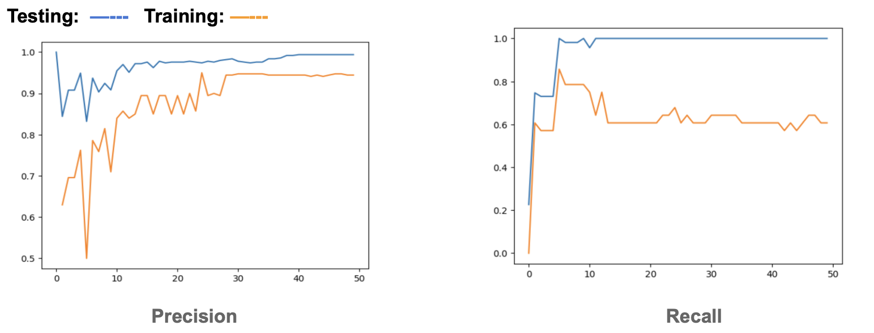
The first parameter is the amount of data that I sampled before training. I am using 10% of the training data every time I train a new classifier. In the process of developing the code I have experimented with several sample sizes. Sample sizes with more that 70% tend to over fit the ensemble. While sample size around 50% will dramatically improve either precision or recall after a point. The problem with sudden improvement is that generally precision tends to go up but recall tends to decline sharply, after a single iteration. I wanted a more gradual increase or decrease in any case. The thought process is that if it improvesgradually, itwouldbeeasiertochooseaspotwhereIcouldtradeoffbetweensomeprecision or recall value I want. Rather than compromising on recall because of sharp increase in precision.

The second parameter to tune was the size of the neural network. It was fairly straight forward. As, the number of sample sizes I am training is only 10% out of the original dataset. I was sure that a deep model will overfit the sample. A shallow Neural Network is sufficiently capable to perform classification. Also, I used L1 regularization to further prevent overfitting on the data. Third parameter tuned is the stopping criteria. As we are using multiple iterations and picking up hard to classify samples with higher probability, it is obvious that the number of active compounds gets picked up more and the recall is taken care of. So I had to make sure that I did not lose precision. So, the early stopping criteria has higher precision [82%] criteria. Another parameter to tune is the learning rate. As my sample size is less, a higher learning rate(0.5) created complete imbalance in the sample set. I observed, sometimes it used to take all active compounds and other times it would take all inactive compounds. Instead, I decided to tradoff lower learning rate with increased ensemble size. For the ensemble size, I decided to put a sufficiently large number and then choose the best size after cross-validation and visualization.

5. Ensemble Size Selection

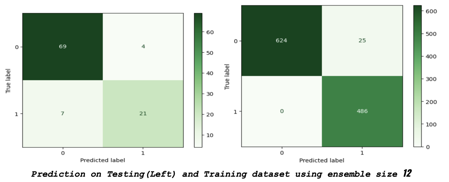
It is evident to choose ensemble size of 12, as it is very accurate. However, there are other candidate answers. I chose 32 as the final ensemble size. Ensemble size 32 has more precision. It misspredicts 3 active compounds in the test set (totaling to 10). But, in the training set there are only 13 miss predictions in inactive compounds. Which means the classifier had to miss predict 12 in-active compounds (in case of size 12) in order to identify . So, this is a bad generalization case. This is the reason to choose ensemble size as 32, because it was able to generalize better. Here, the tradeoff I made for higher precision and a bit lower recall. The confusion matrix of size 32 is in the Jupyter notebook. The final accuracy is 77%. It is to choose the size of the ensemble and the trade off between precision and recall. I tried with an was not accurate. As it is a mean between precision and recall, with super higher precision and lower recall it could show us an average that is good enough but could not give similar results.