Clustering

---
Source Code available in the repository
Github handle: bhaba-ranjan
Project: clustering
Repository: https://github.com/bhaba-ranjan/clustering
---

1. Overview

As described in the problem statement. The given dataset consists of pixel values of digits. The dimension of the data set is 784. They all corresponds to picture of size 28*28 pixels. In two dimensions. The objective is to cluster similar digits together. To achieve the objective several steps were performed. They are broadly categorized into the following.

1. Data Analysis
2. Data Preprocessing
3. Dimensionality Reduction
4. Running K-means clustering and Analysis

2. Data Analysis

So the given dimension of data is 784. Each of this feature represents a number between 0-255 representing their color in the original image of size 2828 pixels. The first thing I tried is to recreate the image based on the gray scale so that I can have an idea of the different digits. As, the original image is of 2828 pixels. I resized it as a 2 dimensional grid. And then visualized it through the cv2 library. I found out that different styles of the same digit exist in the dataset. Some findings are below.

This means that we cannot take the accurate representation of the pixels and achieve good clustering results. Another important finding is that a lot of pixels are 0. For some columns almost all pixels are zero. I have visualization and more discussion about this in the dimensionality reduction section.

3. Data Preprocessing

As from the above analysis, it is clear that plotting direct pixel values in a high dimensional space is not going to add any meaningful value to our clustering algorithm. As the pixel of each digit could vary a lot because of the different style of the same digit.

For this reason I decided to make them more similar. The reason behind this is, if I could make images of the same digit similar by applying some logic they would fall near each other. This would result in better clustering. To be specific, the intra cluster distance will be reduced. It is known that minimizing intra cluster distance results in a better clustering overall.

One way to achieve this is to ignore some features that are very specific to a certain style. By doing this we would achieve a better generalization. As we are less biased towards certain features and looking at the overall construction of images. Overall construction is very similar for a digit, so we could generalize them well and present them near to each other in a high dimensional space.

To achieve this we could use averaging, average takes a n*n grid matrix and averages those pixel values. This window averaging technique is applied for all the pixels in the image. This results in a smoother image. As a result more fine grained details are lost and images start to look similar and cluster near each other for the same digits. I am also using gaussian smoothing in order to remove any gaussian noise. It works the same as averaging but the matrix value is derived from a gaussian curve. After applying this smoothening technique these are the resulting images. As you could notice images are Are now a lot smoother. The sharpness is less and they generalize well in terms of pixel colors.

4. Dimensionality Reduction

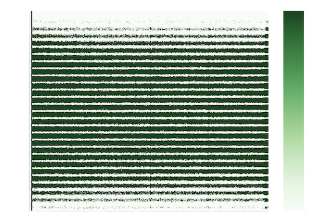
It was not very difficult to spot that we need some reduction in dimension. But choosing the right method and tuning the parameter was very critical for the problem. Initially by just looking at the data I could see a lot of zeros around the first few columns. So, I wanted to check how sparse the data is. In order to understand the features and their representation better, I used a heatmap to visualize how many features actually represent enough colors. On the left the heatmap represents the features on the vertical axis and respective color counts in the horizontal axis.

As we could clearly see from the heatmap that a lot of features do not represent any meaningful color, all of that row is just the lightest color representing 0 for all the colors. Also, the left most column for representing color 0 has the darkest color for all features. Which means almost all features have a lot of pixels with color 0.

4.1 PCA

It is clear from the previous analysis that a lot of the features do not represent any meaningful color. A lot of them have color 0 in excess. It does not make any distinction between. So, I used PCA to reduce redundant features and merge them into one generic feature. This helped a lot in reducing dimension. PCA tries to project the dataset into a hyperplane but it chooses the plane that retains the maximum variance of the data set. In this case Instead of specifying n_component to a specific number. I set it to 0.99 which means to find a hyperplane that preserves 99% variance of the original dataset. I found it to be useful for not losing meaningful details. After running PCA I am able to reduce the dimension of the dataset from 784 down to 86.

4.1 Learning Manifolds

It was one of the most important parts of solving the problem. Learning manifolds is another dimensionality reduction technique. It is a lot different from PCA. While PCA tries to find a hyperplane, manifold learning is about learning a hyperplane which is twisted in the high dimensional space. In general manifold learning projects n dimensional data to d dimension where d < n that resembles

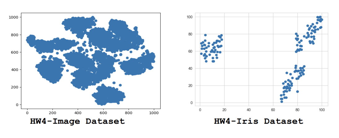
d-dimensional hyperplane locally. We could understand this by using a popular dataset. As we can already see on the rightmost side for swiss roll dataset PCA is not alway the best option if the dataset is twisted. However, manifold captures the property of the data verywell. I am using t-SNE manifold learning technique for further reducing the dimension of the data to 2-Dimension. I am using parameter perplexity set to 19 which looks at the k-neighbor in order to decide between the attention between local and global data. early_exagration is set to 26; this parameter exaggerates the distance between two clusters more than usual. This helps in clustering because we want clusters that are far apart to avoid conflicting data points as much as possible. Based on the perplexity parameter value it could have a different shape. The choice of this value is critical mostly in between 5-50. I tried different smaller and larger values and based on the visualization I kind of did like a binary search to arrive at the right parameters that separates the data in a decent manner.

5. K-Means Clustering

So the main part of the implementation was to initialize centroids so that at least one point is assigned to a centroid. There were instances of bad initialization because all of them were random initialization. But this case has to be handled gracefully. I have tried generating random numbers, but getting random numbers from a data point was a bit better. Because, the centroid would lie within the region of data points. And there are less chances of bad centroid initialization. The pseudo code for the algorithm is as follows.

GenerateKCentorids ( TrainingData, K )

1. mapping_of_k = [ ]
2. For K in range [ 1- K ] a. Random_Index = generate TraningData.Column random number in range [ 1 to number of Training Data.Rows ] b. Add Random_index to mapping_of_k
3. centroids = [ ]
4. For single_array in mapping_of_k a. temporary_hold = [ ] b. For index in range [ 1 to TrainingData.Column ] Add TrainingData[ single_array[index] ] [ index ] to temporary_hold c. add temporary_hold to centroids
5. return centroids While generating initial centroids is a little twisted, implementing K-Means was quite straightforward. Only, one thing to take care about this implementation is re-initializing the centroids if a centroid is unassigned to any data points. Which is considered as a bad initialization case. Pseudo code for K-means is mentioned below.

RunKMeansClustering( K, TrainingData, Centroids )

1. Find euclidean distance between TrainingData and each Centroid
2. Assign Each Data Points to the nearest Centroid and make a respective Bucket for all data points within a cluster.
3. If any Bucket is empty Re-initialize the the Centroids by calling GenerateKCentorids restart from Step 1
4. Find the mean of each Bucket consisting of data points.
5. If the mean of Buckets matches respective centroids. Terminate the algorithm and return the bucket.
6. Else make these means as respective new centroids and re-run from step 1. I am running K-means clustering repeatedly for 400 times with different centroids with a value of K set to
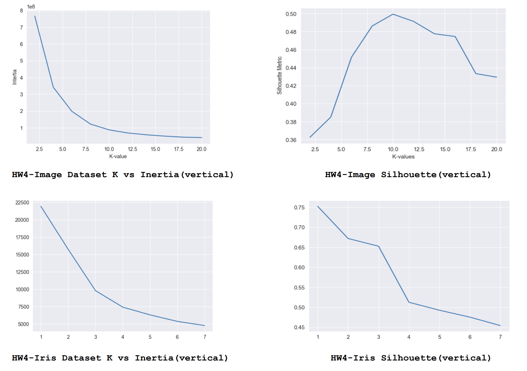
7. For each answer I am calculating the inertia and finally selecting the best centroids based on the lowest inertia score. And before submitting I am adding 1 to each label as the cluster range is from 1 to 10 instead of 0 to 9. I have also tried with different values of K. I have tried values from 2 to 20 in increments of 2. For each K I’m running 10 iterations with different centroid values and finally choosing the best centroid values based on lowest inertia among them. These are the respective scores.

As we could see from this analysis generally the lower inertia with smallest K and and largest Silhouette score gives better results. For K = 10 we get lowest inertia and highest Silhouette score for the Image data set and the same effect could be observed for K=3 in the Iris dataset.