Semantic Segmentation

---
Source Code available in the repository
Github handle: bhaba-ranjan
Project: Semantic Segmentation
Repository: https://github.com/bhaba-ranjan/DeepLabV3
---

1. Introduction

Semantic segmentation is a classical computer vision problem which involves assigning labels or categories to each pixel. Unlike the image classification task which classifies an image overall, image segmentation deals with classifying each pixel to understand the visual content of the image at pixel level. This introduces unique challenges in developing semantic segmentation models. Because, apart from high level understanding, it needs low level understanding and localization to identify where an object is present in an image. Semantic segmentation is used in a variety of applications including autonomous driving and medical imaging. Some of the key application areas are discussed in the following paragraph.

Image segmentation is very popular in various video and image editing applications for automatically outlining borders, object replacement and background removal are some of the key usages. It is heavily used for scene understanding in several applications including robotics, autonomous driving, surveillance systems where accurate perception of the environment is a critical component. Apart from these applications it is also popular in medical imaging for identifying abnormalities in CT and MRI scans. In our work we took a popular semantic segmentation model named DeepLabV3 and tested its adaptation on a different dataset with some popular backbone networks.

2. Related Work

The advent of neural networks has led to significant improvement in the accuracy of semantic segmentation tasks. Most of these learning based algorithms use a lot of classical computer vision concepts in order to achieve fine grained segmentation capabilities. Over time there have been a lot of changes and new components introduced to do semantic segmentation in an accurate and robust manner. Some of the popular work is discussed in this section.

Fully Convolutional Networks (FCN) was introduced in 2014 as one of the preliminary works that used convolutional neural networks to do semantic segmentation. It replaced fully connected layers in the network with upsampling techniques such as interpolation and transposed convolution to restore the spatial resolution in the output. FCN suffered from limited contextual information. In the following year to create more accurate feature maps another paper introduced U-Net [2] which used direct connection from the encoder to improve on the performance by gaining access to some of the high and low level features in the decoder layer. DeepLab was initially introduced in 2014 but improved dramatically in its following incremental improvement iterations (DeepLabV2 and DeepLabv3[3]). The DeepLab model employed several other techniques in addition to the regular encoder-decoder based architecture to improve significantly on several computer vision benchmark datasets. Some of the key details of the DeepLabV3 model are discussed in the following sections.

Another line of work extended the faster R-CNN object detection algorithm by adding a branch for pixel level segmentation. Mask R-CNN are widely popular for tasks that require both object detection and segmentation. One of the other notable lines of work is EfficientNet [4], it focused more on improving efficiency and performance tradeoff in deep learning models. It introduces compound scaling which uniformly scales network depth, width and resolution to find a balance between computational efficiency and accuracy.

3. DeepLabV3 Architecture

In this section we will be discussing some of the key architecture details of DeepLabV3, the thought process behind using them and how they influence the end result of segmenting an image.

Following are some of the key components of DeepLabV3 network that made deeplabV3 accurate and each of these is covered in detail in the following section.

1. Use of dilated convolutions
2. Artous spatial pyramid pooling
3. Conditional random fields

3.1 Dilated Convolution

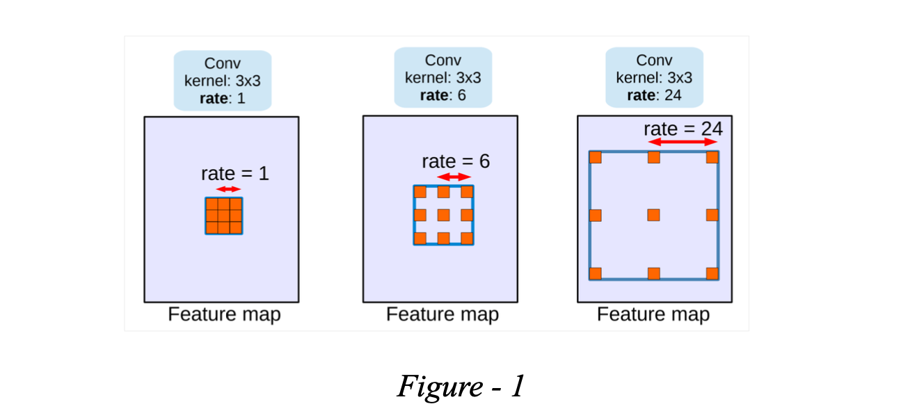
Dilated convolution unlike regular convolution takes an additional parameter known as dilation rate. Dilation rate refers to the spacing between the kernels. With a dilation rate of 1 it is the same as regular convolution without any spacing but as it increases the spacing between the kernels increases. Dilation rate enables capturing information at multiple scales without losing the spatial resolution.

A dilation rate greater than one increases the receptive field by skipping input pixels based on the specified rate. As this method preserves spatial resolution at multiple scales it is a crucial component of image segmentation problems. This property is exploited in DeepLabV3 in different ways; it helps models to learn representation with varying abstraction and details [5] which is extremely important for semantic segmentation tasks. Figure 1 is a pictorial representation of dilated convolution.

3.2 Artous Spatial Pyramid Pooling

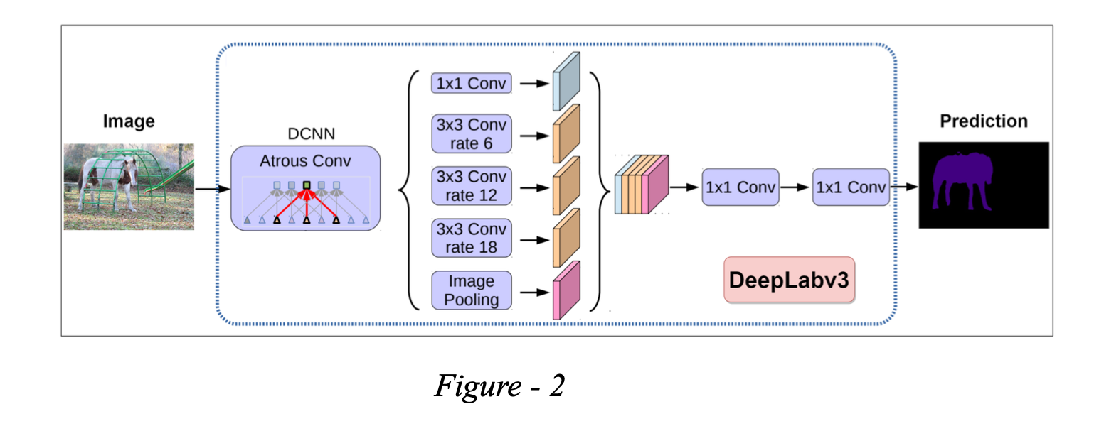
This pooling operation made DeepLabV3 robust at capturing multi-scale contextual information which is an essential part of semantic segmentation. In this paper [6], where parallel atrous convolution is applied with different dilation rates to effectively do semantic segmentation. The paper showed that effective resampling of features at different scales could potentially increase accuracy in identifying images at multiple scales. Following diagram is a depiction of Aspp.

For ASPP DeepLabV3 uses multiple parallel branches, each having a different dilation rate. Number of parallel branches is determined by the scale variation required to extract context. Apart from the number of branches it is crucial to select a proper dilation rate which will capture information and adapt to objects of different sizes in the input image. The output feature maps of the branches are then combined to form a rich feature representation of the image to enable the model to do accurate semantic segmentation. ASPP enabled DeepLabV3 to focus both on fine-grained details and high level context at the same time.

3.3 Conditional Random Fields (CRF)

Although DeepLabV3 is able to outperform most of the contemporary models without CRF, including CRF as a post processing technique could further improve segmented object boundaries. ASPP is successful in covering various receptive fields and capturing fine grained details however the large receptive field and scale variance yield smooth responses. Though this time ASPP significantly improved the image boundary over DeepLabV2 and was able to outperform it in benchmarks. Conditional random fields define an energy function that ensures consistent labelling of neighbouring pixels. It uses two gaussian kernels in different feature spaces; the first bilateral kernel is in pixel position and intensity space while the second one only depends on the pixel position[7].

4. Experimental Setup

In our work we are interested in seeing how the model performs in terms of adapting to a new data set on which it is not trained previously and how it performs for different backbone as feature extractors. We primarily used two backbone networks as feature extractors that are ResNet-50 and MobileNet. The backbones are pre trained on the ImageNet dataset. We took pretrained weights of DeepLabV3 trained on PASCAL VOC 2012 dataset and then fine tuned the model to accommodate for Cityscapes dataset as they have different numbers of classes.

Initial DeepLabV3 has the mIoU of 0.79 for ResNet-50 and 0.7 for MobileNet on PASCAL VOC dataset. Then we trained the model using cross entropy loss. We used SGD stochastic gradient descent for optimization with a learning rate of 0.001 for the DeepLabV3 model and 0.0001 for backbone network with the same optimization technique.

4.1 Experimental Results and Analysis

Initially without any training just with pretrained weights on PASCAL we passed an image from the Cityscape dataset to the network and observed the following output.

It is evident from the initial prediction that the model is able to recognize the object it has seen before in the dataset (PASCAL) it is previously trained on, although the boundaries are not very sharp. As the PASCAL dataset contains instances of cars, pedestrians, buses and cyclists the model is able to recognize them even with the default weights. However, the model could not recognize traffic lights and signs as it has not seen it before in the PASCAL dataset.

After this observation we started training the model on the Cityscape dataset and validated the model on every 5th iteration and kept some of the results to understand how the model is adapting to the new dataset in consequent iterations.

Following are some observations of validation set at different mIoU.

From figure 4 we could see that the IoU goes down as soon as we start training because the model starts adapting to the new colour encoding of the Cityscape dataset. We observed that during validation the model was able to adapt to the objects it has seen before at a much earlier level than the object it has not seen before. As it can be seen the model is able to adapt to pedestrians and cars quickly in the earlier iteration in ResNet-50 mIoU 0.27 and gradually it learns to segment the object it has not seen before like traffic lights and signs which can be seen in MobileNet mIoU 0.4 image.

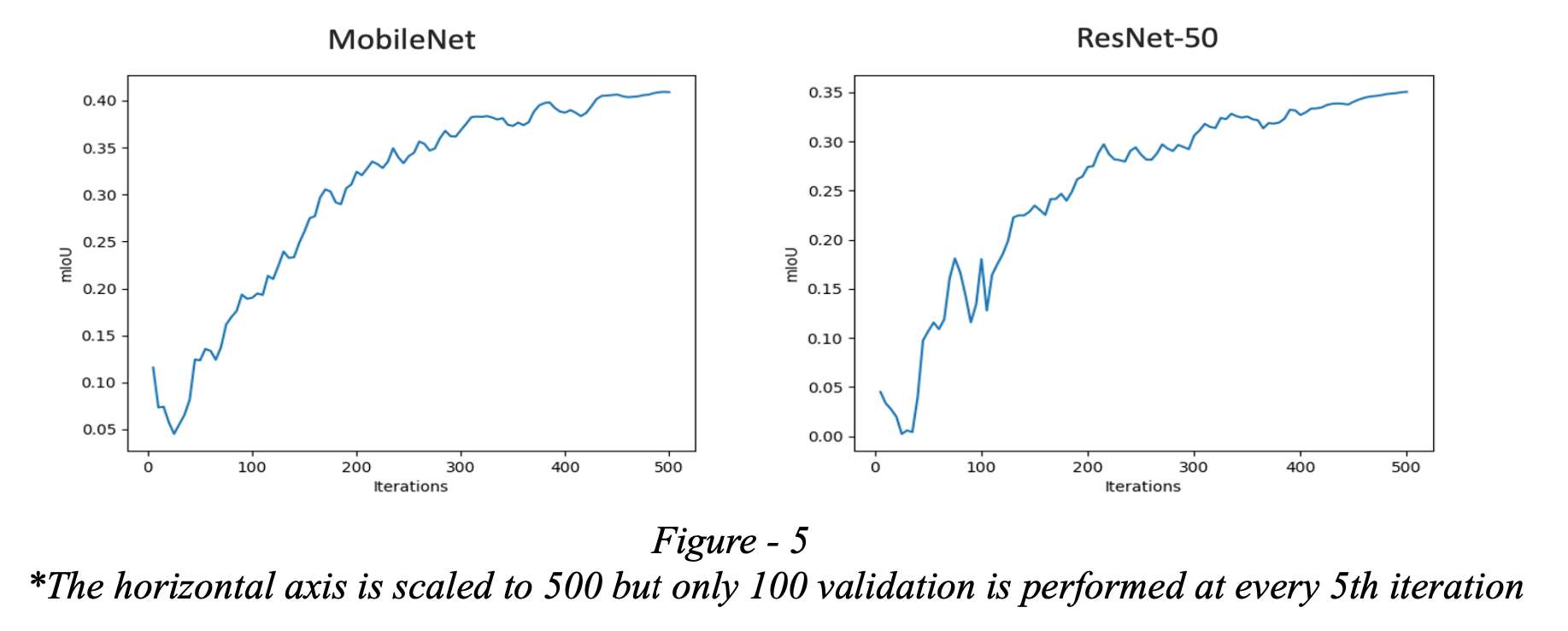
Apart from the adaptation to the image segmentation we also monitored the improvements in mIoU over the validation sets for different networks. The following figure is a depiction of the same.

As it can be seen from the graphs that the mIoU initially drops as the model starts adapting to the new class scheme but as soon as it adopts the new class masks the IoU starts increasing rapidly in the following iterations. Another observation that can be drawn from the graphs is that at each iteration end of the validation set the MobileNet backbone model is able to get higher mIoU scores in most of the cases as compared to the ResNet-50 backbone model. Even in the final iteration, the ResNet-50 model was able to achieve 0.32 in mIoU score but MobileNet reached up to 0.4 in mIoU score. We think that this is because ResNet-50 is larger because of the number of layers; however, MobileNet is much smaller and is designed for devices with low computational resources.

5. Conclusion

In our project we are successfully able to run DeepLabV3 with a different backbone and able to quantify some of the key differences in terms of performance and adaptation to new data. We observed that both of these metrics are influenced by the distribution of data the model is previously trained on as well as the backbone it uses. We also learned that backbone should be chosen carefully according to application requirements, for example for faster inference and low resource devices MobileNet should be used whereas ResNet-50 has the potential to give more accuracy if sufficiently trained. Motivated by our work we further want to run similar analysis on popular models that use transformers for semantic segmentation in our future work